[CS] Image Compression with DHWT

이 글은 이향원 교수님의 선형대수학 강의와 프로젝트를 기반으로 작성되었습니다.
해당 강의의 2014년 녹화본은 여기(KOCW)에서 시청할 수 있으며, 이 글은 해당 강의 기준 6주차 수업을 정리한 글입니다.

0. Introduction - Change of Basis

There are a lot of situations where you have to store matrics. One typical example of this situation is storing an image. Considering that an image can be expressed with 3 2-dimensional matrix, each representing R, G, B channels of the image, it would take enormous amount of storage if you naively store the entire matrix. Instead, we may consider storing the image with the linear combination of pre-determined basis.

Consider $4 \times 4$ image, and let $A$ be the first column of the image. Suppose

\[A = \begin{bmatrix} 2 \\ -2 \\ 2 \\ -2 \end{bmatrix}\]

Using standard basis of $\mathbb{R}^4$, $A$ can be expressed as

\[A = 2\begin{bmatrix} 1 \\ 0 \\ 0 \\ 0 \end{bmatrix} -2\begin{bmatrix} 0 \\ 1 \\ 0 \\ 0 \end{bmatrix} +2\begin{bmatrix} 0 \\ 0 \\ 1 \\ 0 \end{bmatrix} -2\begin{bmatrix} 0 \\ 0 \\ 0 \\ 1 \end{bmatrix}\]

and thus can be represented as quadruple $(2, -2, 2, -2)$. Note that it did not change the size of $A$ at all.

Now consider basis

\[\left\{ \begin{bmatrix} 1 \\ 1 \\ 1 \\ 1 \end{bmatrix}, \begin{bmatrix} 1 \\ -1 \\ -1 \\ 1 \end{bmatrix}, \begin{bmatrix} 1 \\ 1 \\ -1 \\ -1 \end{bmatrix}, \begin{bmatrix} 1 \\ -1 \\ 1 \\ -1 \end{bmatrix} \right\}\]

With this basis, $A$ can be represented as tuple $(4, 2)$, which means 2 times the last vector in the basis.

This shows that if we aim to compress images with linear combination of basis, we need good basis to fully exploit the advantage. We are going to discuss how JPEG standard compresses images using “change of basis.”

1. Backgrounds

1-1. Kronecker Product

For an $m \times n$ matrix $A$ and $p \times q$ matrix $B$, the Kronecker Product

\[A \otimes B\]

is an $np \times mq$ matrix defined as

\[A \otimes B = \begin {bmatrix} a_{11}B & a_{12}B & \dots & a_{1n}B \\ a_{21}B & a_{22}B & \dots & a_{2n}B \\ \vdots & \vdots & \ddots & \vdots \\ a_{m1}B & a_{m2}B & \dots & a_{mn}B \\ \end{bmatrix}\]

For example,

\[\begin{bmatrix} 1 & 2 \\ 3 & 4 \end{bmatrix} \otimes \begin{bmatrix} 1 & 1 \\ 2 & 2 \\ 3 & 3 \end{bmatrix} = \begin{bmatrix} 1 & 1 & 2 & 2 \\ 2 & 2 & 4 & 4 \\ 3 & 3 & 6 & 6 \\ 3 & 3 & 4 & 4 \\ 6 & 6 & 8 & 8 \\ 9 & 9 & 12 & 12 \\ \end{bmatrix}\]

1-2. Haar Matrix

For $n = 2^t$($t \in \mathbb{Z}^{+}$), the $n$-point Haar matrix $H_n$ is an $n \times n$ matrix defined as

\[H_n = \begin{cases} \bigl[\, H_m \otimes \begin{bmatrix} 1 \\[2pt] 1 \end{bmatrix} \;\; I_m \otimes \begin{bmatrix} 1 \\[2pt] -1 \end{bmatrix} \,\bigr], & \text{if } n = 2m, \\[12pt] \begin{bmatrix} 1 \end{bmatrix}, & \text{if } n = 1. \end{cases}\]

2. Discrete Haar Wavelet Transform

JPEG groups image into $8 \times 8$ blocks, and compresses each block separately using $8$-point Haar matrix discussed in the section above. Following the definition recursively, we can construct $8$-point Haar matrix $H_8$ as

\[H_8 = \begin{bmatrix} 1 & 1 & 1 & 0 & 1 & 0 & 0 & 0 \\ 1 & 1 & 1 & 0 & -1 & 0 & 0 & 0 \\ 1 & 1 & -1 & 0 & 0 & 1 & 0 & 0 \\ 1 & 1 & -1 & 0 & 0 & -1 & 0 & 0 \\ 1 & -1 & 0 & 1 & 0 & 0 & 1 & 0 \\ 1 & -1 & 0 & 1 & 0 & 0 & -1 & 0 \\ 1 & -1 & 0 & -1 & 0 & 0 & 0 & 1 \\ 1 & -1 & 0 & -1 & 0 & 0 & 0 & -1 \end{bmatrix}.\]

Noting that all columns are orthogonal, we can easily find that columns of $H_8$ are basis of $\mathbb{R}^8$, as $n$ linearly independent vectors span $\mathbb{R}^n$, making them basis. If we take the normalized form of $H_8$, then $H_8$ is the orthogonal matrix. As inverse of any orthogonal matrix is its transpose, we get $H_8^{-1} = H_8^T$. This will make calculations much faster.

Note. Every $n$-point Haar matrix is orthonormal when it is normalized. We observed this with $B_8$, but we are going to skip proof.

2-1. Compression

Let $A$ be $n \times n$ matrix where $n$ is the power of $2$. Then its 2-dimensional discrete haar wavelet transform $B$ is

\[\begin{aligned} B &= H_n^TAH_n \\ &= \begin{bmatrix} h_1^T \\ h_2^T \\ \vdots \\ h_n^T \end{bmatrix} A \begin{bmatrix} h_1 & h_2 & \dots & h_n \end{bmatrix} = \begin{bmatrix} h_1^T \\ h_2^T \\ \vdots \\ h_n^T \end{bmatrix} \begin{bmatrix} Ah_1 & Ah_2 & \dots & Ah_n \end{bmatrix} \\ &= \begin{bmatrix} h_1^TAh_1 & h_1^TAh_2 & \dots & h_1^TAh_n \\ h_2^TAh_1 & h_2^TAh_2 & \dots & h_2^TAh_n \\ \vdots & \vdots & \ddots & \vdots \\ h_n^TAh_1 & h_n^TAh_2 & \dots & h_n^TAh_n \end{bmatrix} \end{aligned}\]

The top left corner of $B$ is called “high frequency” component of $A$, which means it holds the most meaningful information of original matrix $A$. This leads us to $\hat{B}$, which is the truncated matrix of $B$. $\hat{B}$ is $m \times m$ matrix from the top left corner of $B$. We are going to store $\hat{B}$ instead of $A$, which saves space if $m \lt n$. Smaller $m$ means higher compression rate, and vice versa (lossy compression). If $m=n$, then it is lossless compression.

2-2. Decompression

We have to expand $\hat{B}$ to $n \times n$ so that we can multiply $H_n$. This can be done by filling in zeros. With zero-filled $n \times n$ matrix $B$, its inverse discrete haar wavelet transform $\hat{A}$ is

\[\hat{A} = H_n\hat{B}H_n^T.\]

Note that if $m=n$ (therefore lossless compression), we can observe that

\[B = H_n^TAH_n\]

and

\[\begin{aligned} \hat{A} &= H_nH_n^TAH_nH_n^T \\ &= I A I \qquad (\because H_n \text{is orthogonal matrix}) \\ &= A \end{aligned}\]

3. Observations

3-1. Impact of $m$ on compressed image

From top left: original, $m=512, 256, 128, \dots, 8$

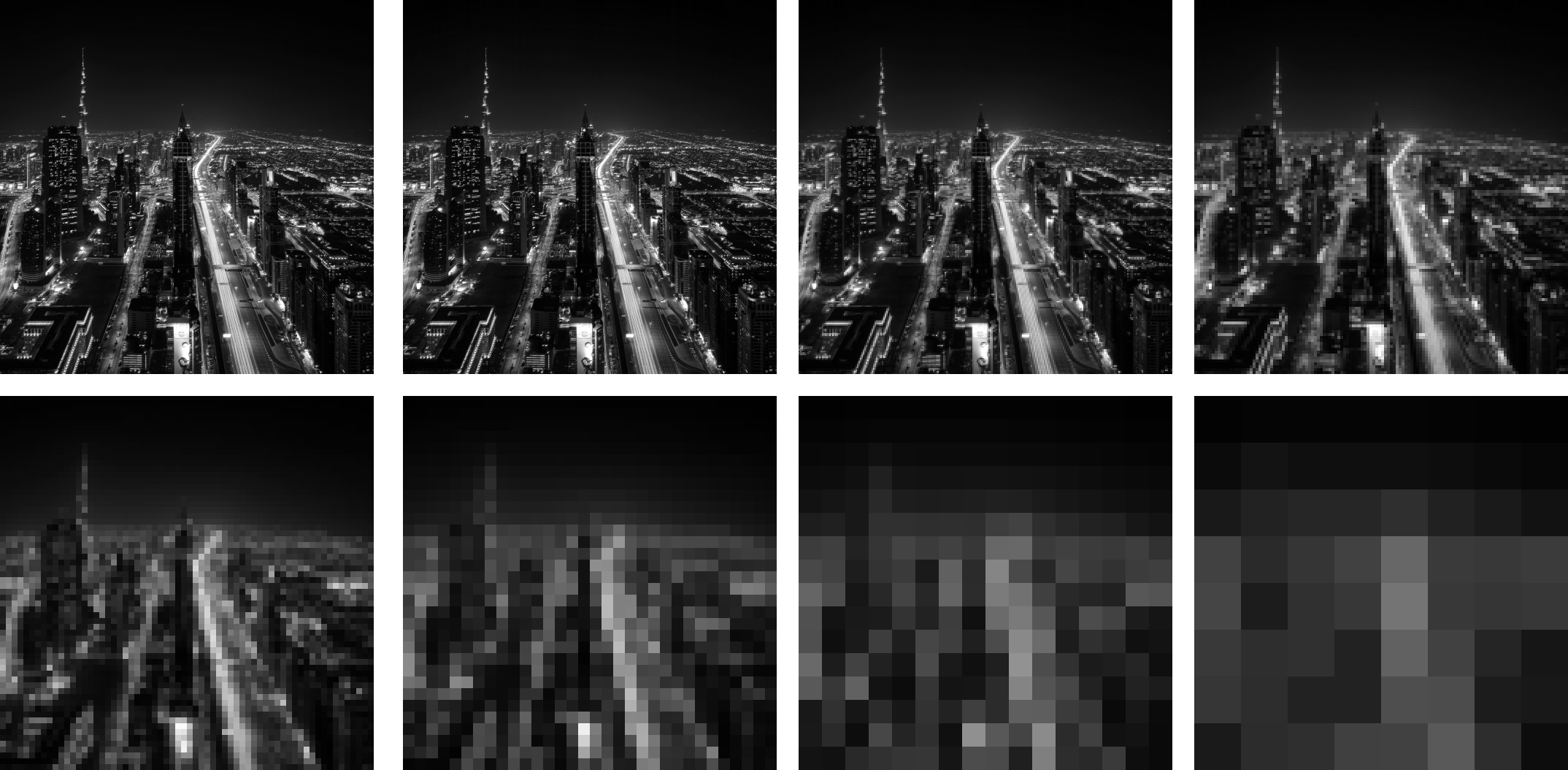
As $m$ increases, the quality of the compressed image improves, as seen in figures above. Notably, when $m$ equals the size of the original image, the compressed image is identical to the original.

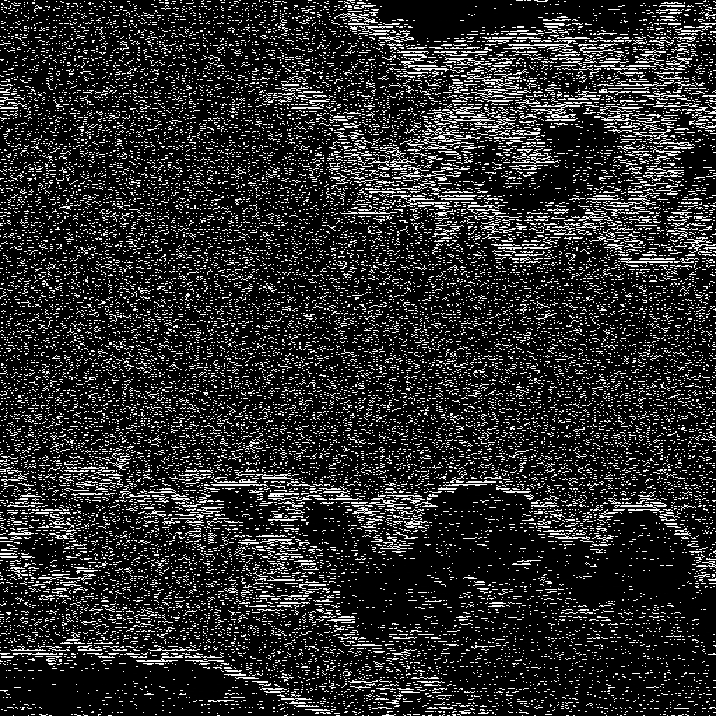
Focusing on the night sky image, the boundary between the sky and ground(a relatively low-frequency region) reveals that image quality is maintained even as $m$ decreases. However, observing the city area, a relatively high-frequency region, , shows that quality drops sharply even with a slight decrease in $m$. (Focus on the building lights; we can barely see the lights coming from building’s windows from $m=128$.)

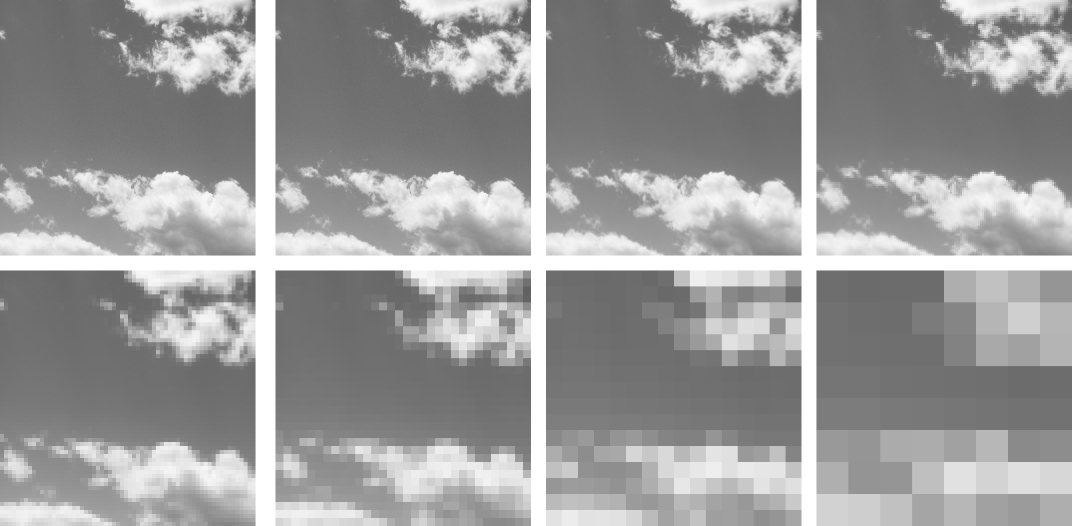
Similarly, in the sky image, examining the relatively low-frequency regions like the sky and the interior of the clouds shows that image quality is maintained even as $m$ decreases. Particularly in the sky region, there is almost no change, so even at $m=32$. However, looking at the relatively high-frequency region at the boundary between the clouds and the sky, as seen above, it can be observed that even a slight decrease in $m$ causes a sharp drop in quality. In particular, the small clouds at the cloud edges completely disappear around $m=16$.

3-2. Focusing on high and low components of $H$

Let $n$-point normalized Haar matrix $H$ is given as

\[H^T = \begin{bmatrix} H_l \\ H_h \end{bmatrix}\]

so

\[H = \begin{bmatrix} H_l^T & H_h^T \end{bmatrix}.\]

Then, DHWT B is,

\[\begin{aligned} B &= H^{T} A H \\[4pt] &= \begin{bmatrix} H_l \\ H_h \end{bmatrix} A \begin{bmatrix} H_l^{T} & H_h^{T} \end{bmatrix} \\[6pt] &= \begin{bmatrix} H_l A \\ H_h A \end{bmatrix} \begin{bmatrix} H_l^{T} & H_h^{T} \end{bmatrix} \\[6pt] &= \begin{bmatrix} H_l A H_l^{T} & H_l A H_h^{T} \\ H_h A H_l^{T} & H_h A H_h^{T} \end{bmatrix}. \end{aligned}\]

If we perform IDHWT on B,

\[\begin{aligned} A &= H B H^{T} \\[4pt] &= \begin{bmatrix} H_l^{T} & H_h^{T} \end{bmatrix} \begin{bmatrix} H_l A H_l^{T} & H_l A H_h^{T} \\ H_h A H_l^{T} & H_h A H_h^{T} \end{bmatrix} \begin{bmatrix} H_l \\ H_h \end{bmatrix} \\[6pt] &= \begin{bmatrix} H_l^{T} H_l A H_l^{T} + H_h^{T} H_h A H_l^{T} & H_l^{T} H_l A H_h^{T} + H_h^{T} H_h A H_h^{T} \end{bmatrix} \begin{bmatrix} H_l \\ H_h \end{bmatrix} \\[6pt] &= H_l^{T} H_l A H_l^{T} H_l + H_h^{T} H_h A H_l^{T} H_l + H_l^{T} H_l A H_h^{T} H_h + H_h^{T} H_h A H_h^{T} H_h . \end{aligned}\]

Visualize each term with image, and we get

$H_h^T H_h A H_h^T H_h$

$H_h^T H_h A H_l^T H_l$

$H_l^T H_l A H_h^T H_h$

$H_l^T H_l A H_l^T H_l$

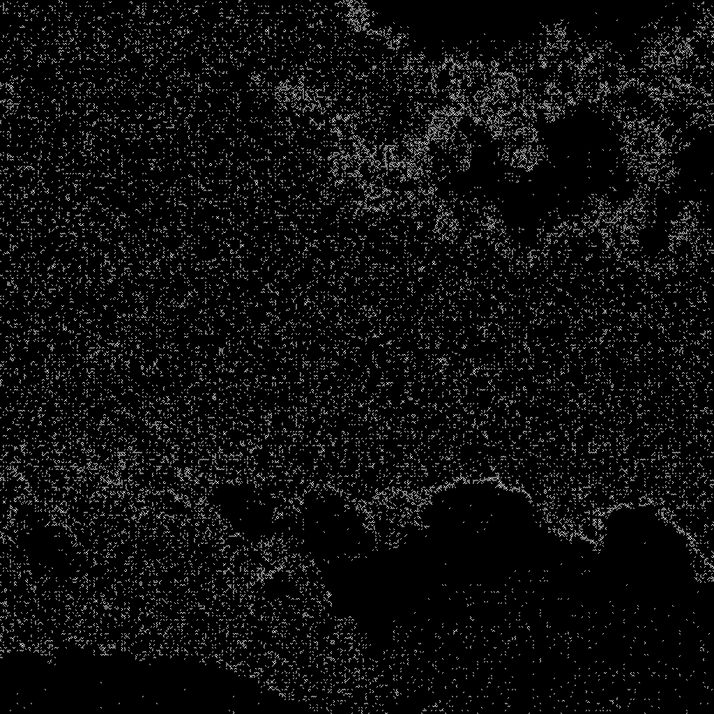
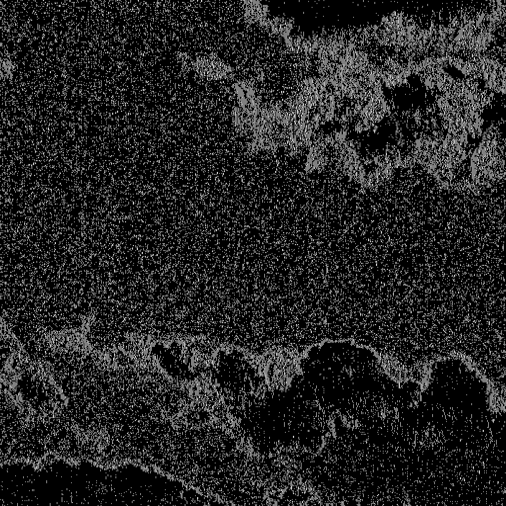
Focusing on the boundary between sky and cloud (which is high-frequency section of the image), we can interpret each term as

• $H_h^TH_hAH_h^TH_h$ represents changes in the diagonal components.
• $H_h^TH_hAH_l^TH_l$ represents changes in the vertical components.
• $H_l^TH_lAH_h^TH_h$ represents changes in the horizontal components.
• $H_l^T H_l A H_l^T H_l$ is the compressed version of the image.

4. Accelerating Calculation with $P_{p, r}$

이 부분의 내용은 Golub & Van Loan, Matrix Computations 의 1.4 Fast Matrix-Vector Products - Algorithm 1.4.4 내용과 연관있습니다.

The mod-p perfect shuffle permutation $P_{p,r}$ treats the components of the input vector $x \in \mathbb{R}^n$, $n = pr$, as cards in a deck. The deck is cut into $p$ equal “piles” and reassembled by taking one card from each pile in turn. For example, if p = 3 and r = 4, then the piles are $x(1:4)$, $x(5:8)$ , and $x(9:12)$ and

\[P_{3, 4}\mathbf{x} = \begin{bmatrix} \mathbf{x}(1:4:12) \\ \mathbf{x}(2:4:12) \\ \mathbf{x}(3:4:12) \\ \mathbf{x}(4:4:12) \\ \end{bmatrix} = \begin{bmatrix} x_1 \\ x_5 \\ x_9 \\ x_2 \\ x_6 \\ x_{10} \\ x_3 \\ x_7 \\ x_{11} \\ x_4 \\ x_8 \\ x_12 \\ \end{bmatrix}\]

---

Lemma. $P_{p, r}^T = P_{r, p}$

Intuitive Proof. Considering that $P_{p, r}$ is a permutation matrix, it follows that $P_{p, r}^{-1} = P_{p, r}^T$. We want to show $P_{p, r}^T=P_{r, p}$ and with the fact discussed above, we can pivot this to proving $P_{p, r}^{-1}=P_{r, p}$.

Let $\mathbf{x}$ be a $n(=pr)$ column vector. Then

\[P_{p, r}\mathbf{x} = \begin{bmatrix} \mathbf{x}(1:r:n) \\ \mathbf{x}(2:r:n) \\ \mathbf{x}(3:r:n) \\ \dots \\ \mathbf{x}(r:r:n) \\ \end{bmatrix} := \mathbf{y}.\]

Multiplying $P_{r, p}$ on $\mathbf{y}$ gives

\[P_{r, p}\mathbf{y} = \begin{bmatrix} \mathbf{y}(1:p:n) \\ \mathbf{y}(2:p:n) \\ \mathbf{y}(3:p:n) \\ \dots \\ \mathbf{y}(p:p:n) \\ \end{bmatrix}.\]

Now let’s carefully consider the properties of $\mathbf{y}$. Since $\mathbf{y}$ is ultimately formed by sequentially taking one element at a time from each of the $p$ vectors obtained by partitioning $\mathbf{x}$, it is easy to see that consecutive terms appear every $r$th term. For example, consider the $P_{3, 4}$ given as an example above. By reading each term of $P_{3,4}\mathbf{x}$ sequentially while skipping every fourth term, we can easily observe that we obtain the original vector $\mathbf{x}$.

That is, reading $\mathbf{y}$ by skipping every $r$th element allows the original vector to be reconstructed. Considering that performing this operation is the role of $P_{r, p}$, by the definition of the inverse matrix, $P_{p, r}^{-1}=P_{r, p}$. Combining this with the result discussed at the beginning, we see that $P_{p, r}^T=P_{r, p}$, completing the proof. $\blacksquare$

---

Step 1. Show

\[P_{2, m}^TH_n = (H_2 \otimes I_m) \begin{bmatrix} H_m & 0 \\ 0 & I_m \end{bmatrix}\]

Proof.

\[\begin{aligned} P_{2,m}^{T} H_n &= P_{m,2} H_n \qquad (\because\ \text{lemma}) \\ &= P_{m,2} \begin{bmatrix} H_m \otimes \begin{bmatrix} 1 \\ 1 \end{bmatrix} & I_m \otimes \begin{bmatrix} 1 \\ -1 \end{bmatrix} \end{bmatrix} \\[6pt] &:= \mathbf{Y}. \end{aligned}\]

Now, let us focus on $H_m \otimes \begin{bmatrix} 1; \ 1 \end{bmatrix}$. Carefully considering how the Kronecker product is computed, we can easily see that the resulting matrix is simply a copy of each row of $H_m$ duplicated twice. Similarly, for $I_m \otimes \begin{bmatrix} 1; \ -1 \end{bmatrix}$, we can see that it creates a matrix by copying each row of $I_m$ twice and then changing the sign of the second copied row.

From the discussion in lemma’s proof, we can interpret $P_{p, n}$ as writing the original vector by skipping every $n$th entry. Applying this to $\mathbf{Y}$ means that $\mathbf{Y}$ is generated by skipping every $2$nd row of $\begin{bmatrix} H_m \otimes \begin{bmatrix} 1 ;\ 1 \end{bmatrix} & I_m \otimes \begin{bmatrix} 1; \ -1 \end{bmatrix} \end{bmatrix}$, therefore,

\[\begin{aligned} \mathbf{Y} = \begin{bmatrix} H_m & I_m \\ H_m & -I_m \end{bmatrix} &= \begin{bmatrix} I_m H_m & I_m I_m \\ I_m H_m & - I_m I_m \end{bmatrix} \\[6pt] &= \begin{bmatrix} I_m & I_m \\ I_m & - I_m \end{bmatrix} \begin{bmatrix} H_m & 0 \\ 0 & I_m \end{bmatrix} \\[6pt] &= \left( \begin{bmatrix} 1 & 1 \\ 1 & -1 \end{bmatrix} \otimes I_m \right) \begin{bmatrix} H_m & 0 \\ 0 & I_m \end{bmatrix} \\[6pt] &= \left( H_2 \otimes I_m \right) \begin{bmatrix} H_m & 0 \\ 0 & I_m \end{bmatrix} \qquad \blacksquare \end{aligned}\]

---

Step 2. For $x \in \mathbb{R}^n$ ($n = 2m$), let $\mathbf{x}_T = \mathbf{x}(1:m)$ and $\mathbf{x}_B = \mathbf{x}(m+1:n)$. Show

\[\mathbf{y} = H_n\mathbf{x} = P_{2, m} \begin{bmatrix} H_m\mathbf{x}_T + \mathbf{x}_B \\ H_m\mathbf{x}_T - \mathbf{x}_B \\ \end{bmatrix}.\]

Proof. Multiplying $\mathbf{x}=\begin{bmatrix} \mathbf{x}_T;
\mathbf{x}_B \end{bmatrix}$ on both side gives

\[\begin{aligned} P_{2,m}^{T} H_n \mathbf{x} &= (H_2 \otimes I_m) \begin{bmatrix} H_m & 0 \\ 0 & I_m \end{bmatrix} \begin{bmatrix} \mathbf{x}_T \\ \mathbf{x}_B \end{bmatrix} \\[6pt] &= \begin{bmatrix} I_m & I_m \\ I_m & - I_m \end{bmatrix} \begin{bmatrix} H_m \mathbf{x}_T \\ \mathbf{x}_B \end{bmatrix} \\[6pt] &= \begin{bmatrix} H_m \mathbf{x}_T + \mathbf{x}_B \\ H_m \mathbf{x}_T - \mathbf{x}_B \end{bmatrix}. \end{aligned}\]

By lemma,

\[H_n\mathbf{x}=P_{2, m}\begin{bmatrix} H_m\mathbf{x}_T+\mathbf{x}_B \\ H_m\mathbf{x}_T-\mathbf{x}_B \end{bmatrix} = \mathbf{y}\]

Therefore,

\[\begin{align} \mathbf{y}(1:2:n) &= H_m \mathbf{x}_T + \mathbf{x}_B, \\ \mathbf{y}(2:2:n) &= H_m \mathbf{x}_T - \mathbf{x}_B. \qquad \blacksquare \end{align}\]

---

Focusing on $H_m\mathbf{x}_T$ from the result above, we can recursively expand it until the split $\mathbf{x}_T’$ becomes a two-dimensional column vector. Since the length is halved at each step, the recursion depth of this expansion is $O(\lg n)$ when $\mathbf{x} \in \mathbb{R}^n$. Furthermore, since $m$ is always 1 in $H_m$ when the recursion terminates, there is no need to construct the Haar matrix. Thus, at recursion level $k$, the time complexity for computing $H_m \mathbf{x}_T \pm \mathbf{x}_B$ is $O\left(\frac{n}{2^k}\right)$.

Similarly, when multiplying $P_{2, m}$, if we approach this operation not as multiplying a permutation matrix but as constructing a matrix by skipping every other element (discussed in the proof of lemma), we see that the time complexity is also $O(\frac{n}{2^k})$. Therefore, the overall time complexity of the algorithm is

\[O(\log n + \frac{n}{2^0} + \frac{n}{2^1} + \dots + \frac{n}{2^k}) = O\!\left(\log n + \frac{1 - 2^{-(k+1)}}{1 - 2^{-1}}\, n\right) \sim O(n).\]

Considering that naive multiplication of $H_n\mathbf{x}$ takes $O(n^2)$ time, it provides significantly faster algorithm for performing discrete haar wavelet transform.