[CS] Gradient Descent

0. Introduction

Gradient descent comes from finding $x$ such that

\[\min_{x \in \mathbb{R}^n}f(x)\]

where $f: \mathbb{R}^n \rightarrow \mathbb{R}$

For understanding, suppose $n = 1$, and $f(x) = x^2+2x+4$. As $f$ is a polynomial function (thus differentiable) we can differentiate the function and find $x$s which satisfy $\frac{df}{dx}=0$. However, as $n$ grows, it becomes harder to find local/global minimum points only with this approach. To tackle this, gradient descent proposes method to gradually approach the local minimum points.

1. Backgrounds

2-1. Taylor’s Theorem

For twice continuously differentiable $f: \mathbb{R} \rightarrow \mathbb{R}$, $f$ can be approximated as

\[f(x) \approx f(a) + f'(a)(x - a)\]

as $|x-a| \sim 0$.

The same applies to $f: \mathbb{R}^n \rightarrow \mathbb{R}$. If $f$ is twice continuously differentiable, $f$ can be approximated as

\[f(\mathbf{x}) = f(\mathbf{a}) + \nabla f(\mathbf{a})^T(\mathbf{x} - \mathbf{a})\]

as $|\mathbf{x}-\mathbf{a}| \sim 0$. (Note that both $\mathbf{x}$ and $\mathbf{a}$ are in $\mathbb{R}^n$.)

2-2. Matrix Norms - Induced Norms

For $m \times n$ matrix $A$, $||A||$ is defined as

\[\|A\| = \max_{\mathbf{x} \neq \mathbf{0}} \frac{\|A\mathbf{x}\|}{\|\mathbf{x}\|}\]

this definition can be further reduced as

\[\begin{aligned} &= \max_{\mathbf{x} \neq \mathbf{0}} \left\| A \cdot \frac{\mathbf{x}}{\|\mathbf{x}\|} \right\| \\ &= \max_{\|\mathbf{x}\|=1} \|A\mathbf{x}\|. \end{aligned}\]

We now will focus on calculating the induced norm.

---

Background. Let $A$ be $n \times n$ symmetric matrix (thus diagonalizable). Suppose $\lambda(A) = \{\lambda_1, \lambda_2, \dots, \lambda_n\}$ and without loss of generality, $\lambda_1 \le \lambda_2 \le \dots \le \lambda_n$. Then, $A$ can be diagonalized as

\[A = Q \Lambda Q^T\]

where

\[\Lambda = \begin{bmatrix} \lambda_1 & 0 & \dots & 0 \\ 0 & \lambda_2 & \dots & 0 \\ \vdots & \vdots & \ddots & \vdots \\ 0 & 0 & \dots & \lambda_n \end{bmatrix}\]

and $Q = \begin{bmatrix} \mathbf{q}_1 & \mathbf{q}_2 & \dots & \mathbf{q}_n \end{bmatrix}$ is the matrix of orthonormal eigenvectors. (Note that for orthogonal matrix $Q$, $Q^{-1}=Q^T$)

Lemma. $A^T A$ is positive semidefinite.

Proof. Multiplying $\mathbf{x}^T$ on the left side and $\mathbf{x}$ on the right side gives

\[\begin{aligned} \mathbf{x}^T A^T A \mathbf{x} &= (A\mathbf{x})^T A \mathbf{x} \\ &= \|A\mathbf{x}\|^2 \ge 0 \qquad \blacksquare \end{aligned}\]

Theorem. $||A|| = \sigma_{\text{max}}(A)$, where $\sigma$ is the singular value of $A$.

Proof. The induced norm of $A$ can be rewritten as

\[\begin{aligned} \|A\| &= \max_{\|\mathbf{x}\| = 1} \|A\mathbf{x}\| \\ &= \max_{\|\mathbf{x}\| = 1} \sqrt{\mathbf{x}^T A^T A \mathbf{x}} \\ &= \max_{\|\mathbf{x}\| = 1} \sqrt{\mathbf{x}^T Q \Lambda Q^T \mathbf{x}} \qquad (\because \text{lemma}) \\ &= \max_{\|\mathbf{x}\| = 1} \sqrt{\sum_{i=1}^n\lambda_i(\mathbf{q}_i^T\mathbf{x})^2} \end{aligned}\]

Focusing on $\sum_{i=1}^n(\mathbf{q}_i^T\mathbf{x})^2$, we can easily show that

\[\sum_{i=1}^n(\mathbf{q}_i^T\mathbf{x})^2 = 1\]

as

\[Q^T \mathbf{x} = \begin{bmatrix} \mathbf{q}_1^T\mathbf{x} \\ \mathbf{q}_1^T\mathbf{x} \\ \dots \\ \mathbf{q}_n^T\mathbf{x} \end{bmatrix}\]

and

\[\|Q^T\mathbf{x}\| = \|x\| = 1.\]

Since $\lambda_1 \ge \lambda_2 \ge \dots \ge \lambda_n$

\[\begin{aligned} \max_{\|\mathbf{x}\| = 1} \sqrt{\sum_{i=1}^n\lambda_i(\mathbf{q}_i^T\mathbf{x})^2} &= \sqrt{\lambda_{\text{max}}} \\ &= \sigma_{\text{max}} \qquad \blacksquare \end{aligned}\]

This completes the proof.

2. Idea

2-1. On $f: \mathbb{R} \rightarrow \mathbb{R}$

The idea of gradient descent is quite simple. First, it randomly selects $x_0$ in $\mathbb{R}$ (which is the domain of $f$) and applies following steps:

\[x_{k+1} = \begin{cases} x_k + w, & \text{if } f'(x_k) < 0, \\ x_k - w, & \text{if } f'(x_k) > 0. \end{cases}\]

where $w$ is a positive real number.

The above equation can be interpreted in plain English as follows,

If $f$ is decreasing, move forward.
If $f$ is increasing, move backward.

Following these steps with the function discussed on introduction, we can easily find that $x$ approaches $-1$, which is the local and global minimum point of $f$. We will call this specific value of $x$ (which minimize the function $f$) as $x^*$.

2-2. Expand to $f: \mathbb{R}^n \rightarrow \mathbb{R}$

From the results discussed above, considering that $x$ is moving in the opposite direction of the slope, the following expansion is possible.

\[\mathbf{x}_{k+1} = \mathbf{x}_k - \alpha \nabla f(\mathbf{x}_k)\]

We call positive real number $\alpha$ as “step size” or “learning rate”. (Generally, $\alpha$ is the function of $k$. For simplicity, we suppose that $\alpha$ is fixed.)

3. Proof

For gradient descent to work, we must prove that

\[f(\mathbf{x_k}) \gt f(\mathbf{x_{k+1}}).\]

Suppose a twice continuously differentiable function $f$, and recall

\[f(\mathbf{x}) \approx f(\mathbf{a}) + \nabla f(\mathbf{a})^T(\mathbf{x} - \mathbf{a})\]

substitute $\mathbf{x}$ with $\mathbf{x}_{k+1}$ and $\mathbf{a}$ with $\mathbf{x}_k$ and we get

\[\begin{aligned} f(\mathbf{x}_{k+1}) &\approx f(\mathbf{x}_k) + \nabla f(\mathbf{x}_k)^T(\mathbf{x}_{k+1} - \mathbf{x}_k) \\ &= f(\mathbf{x}_k) + \nabla f(\mathbf{x}_k)^T(\mathbf{x}_{k} - \alpha \nabla f(\mathbf{x}_k) - \mathbf{x}_k) \\ &= f(\mathbf{x}_k) - \alpha \|\nabla f(\mathbf{x}_k)\|^2 \\ \end{aligned}\]

Considering that the $l_2$-norm of a vector is nonnegative and learning rate is always positive, we can deduce that

\[f(\mathbf{x_k}) \gt f(\mathbf{x_{k+1}}) \qquad \blacksquare\]

This completes the proof.

4. Convergence Rate Analysis for Quadratic Cost Functions

For symmetric positive definite matrix $A$, let $f(\mathbf{x}) = \frac{1}{2} \mathbf{x}^T A \mathbf{x}$ (quadratic cost function). Applying GD gives

\[\begin{aligned} \mathbf{x}_{k+1} &= \mathbf{x} - \alpha \nabla f(\mathbf{x}_k) \\ &= \mathbf{x} - \alpha A \mathbf{x}_k \qquad (\text{Note that} \nabla f(\mathbf{x}) = A \mathbf{x}) \\ &= (I - \alpha A)\mathbf{x}_k \end{aligned}\]

Then take the norm on both sides and square it,

\[\begin{aligned} \|\mathbf{x}_{k+1}\| &= \|(I - \alpha A)\mathbf{x}_k\|^2 \\ &\le \|(I - \alpha A)\|^2\|\mathbf{x}_k\|^2 \dots \text{(1)} \end{aligned}\]

We are now going to focus on $I - \alpha A$.

Suppose $\lambda(A) = \{\lambda_1, \dots, \lambda_n\}$, and without loss of generality, $\lambda_1 \le \dots \le \lambda_n$. As $(I - \alpha A)$ is also symmetric, its eigenvalues are all real. Then,

\[\begin{aligned} (I - \alpha A)\mathbf{x} &= \mathbf{x} - \alpha A \mathbf{x} \qquad (\text{x is eigenvector of A}) \\ &= (1 - \alpha \lambda)\mathbf{x} \end{aligned}\]

This shows that $(I - \alpha A)$ has eigenvalues $1-\alpha \lambda$. So,

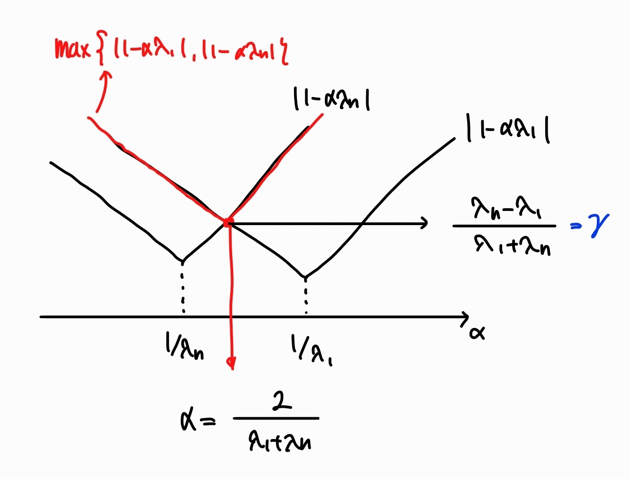
\[\begin{aligned} \|(I - \alpha A)\|^2 &= \max{\{(1 - \alpha \lambda_1)^2, (1 - \alpha \lambda_n)^2\}} \\ &=: \gamma \end{aligned}\]

Then, $(1)$ becomes

\[\|\mathbf{x}_{k+1}\|^2 \le \gamma \|\mathbf{x}_k\|^2\] \[\therefore \|\mathbf{x}_{k}\| \le \gamma^k \|\mathbf{x}_0\|\]

The figure below shows that $\gamma$ has its minimum value $\frac{\lambda_n - \lambda_1}{\lambda_n + \lambda_1}$ when $\alpha = \frac{2}{\lambda_1 + \lambda_n}$.